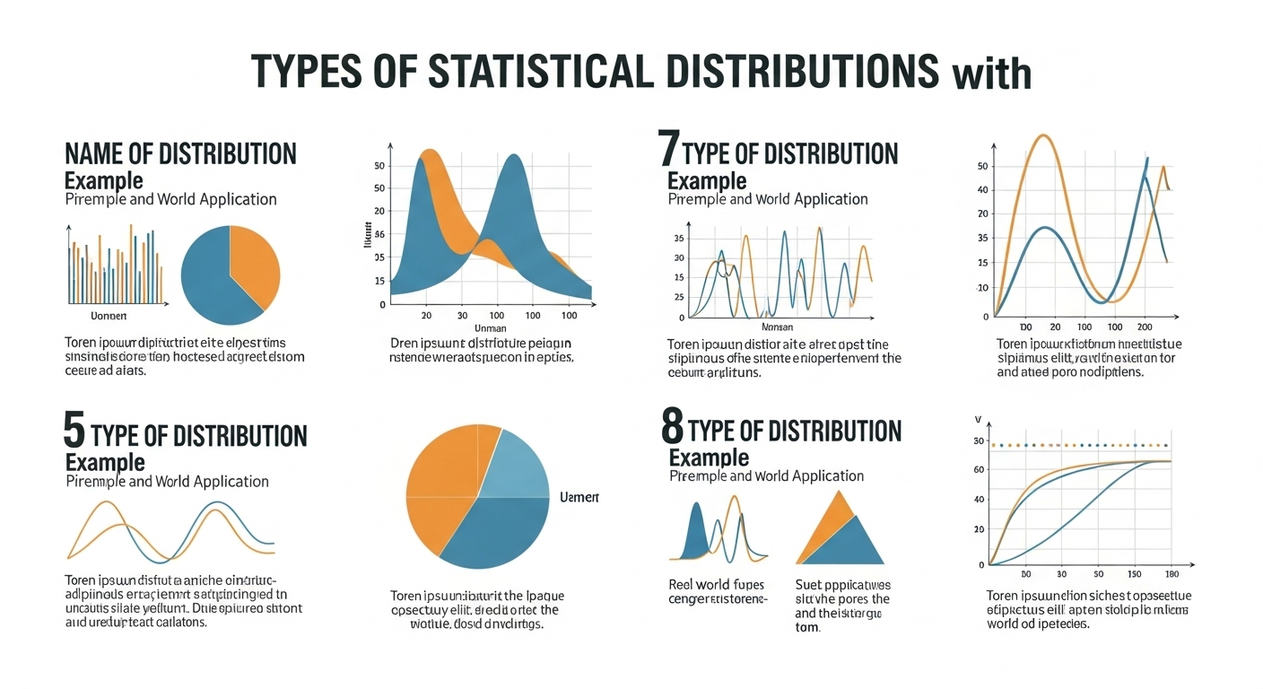
7 Types of Statistical Distributions with Examples and Real-World Applications
Written By David
Lorem ipsum dolor sit amet consectetur pulvinar ligula augue quis venenatis.
Statistical distributions are everywhere in our daily lives. When you flip a coin, check exam scores, or analyze business data, you’re dealing with these patterns. Understanding them helps make better decisions with data.
Data scientists use these tools to predict outcomes and solve problems. Each distribution tells a different story about how information behaves. Let’s explore seven key types that appear most often in real situations.
Understanding Normal Distribution: The Bell Curve in Data Science
The normal distribution creates a bell-shaped curve that’s symmetric around the middle. Most values cluster near the center, with fewer values at the extremes. This pattern shows up in nature constantly.
Think about people’s heights in a country. Most folks are average height, with fewer very tall or very short people. Test scores often follow this same pattern. The bell curve appears in measurement errors too.
Two numbers describe this distribution completely: the average and how spread out the values are. About 68% of data falls within one standard deviation of the mean. This rule helps predict where most values will land.
Many statistical tests assume your data follows this pattern. It’s the foundation for confidence intervals and hypothesis testing. The bigger your sample gets, the more likely averages will follow this shape.
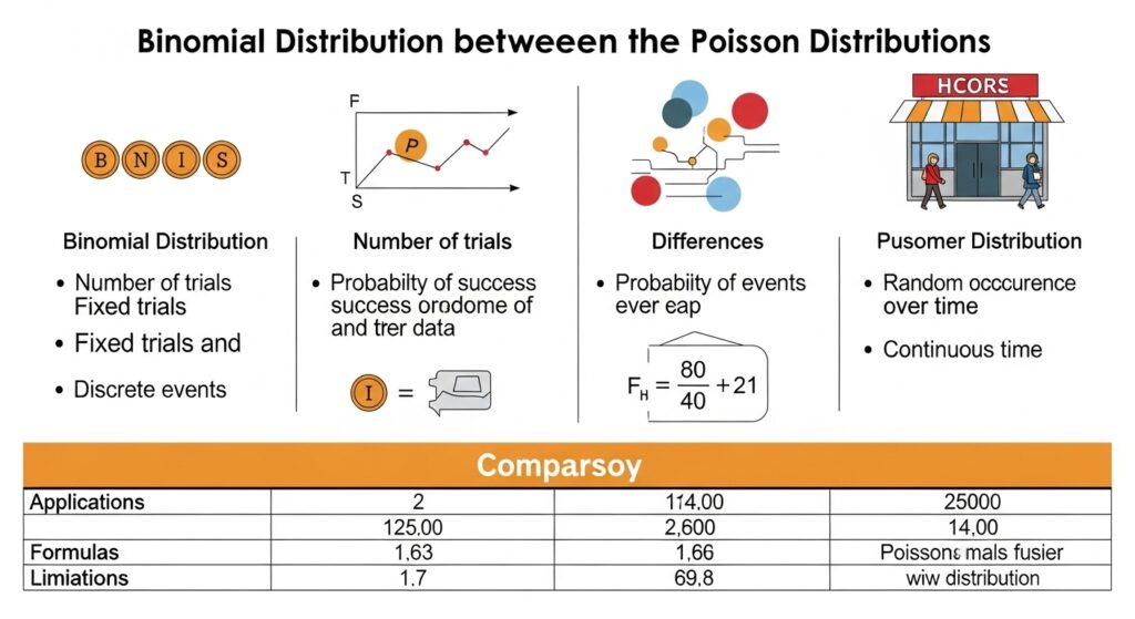
Binomial vs Poisson Distribution: Key Differences Explained
Binomial distribution counts successes in a fixed number of tries. Each attempt has two possible outcomes, like heads or tails. You need to know how many attempts and the success probability.
Poisson distribution counts events happening over time or space. Unlike binomial, you don’t need a fixed number of attempts. It only needs one number: the average rate of events.
Here’s the key difference: binomial has fixed trials, while Poisson works with time periods. Both handle counting, but serve different purposes. Binomial works for surveys, while Poisson fits customer arrivals.
Exponential Distribution Applications in Real-World Scenarios
Exponential distribution models waiting times between events. It’s perfect for predicting when things will happen next. Customer service calls, equipment failures, and radioactive decay all follow this pattern.
The special thing about this distribution is its “memoryless” property. The chance of something happening doesn’t depend on how long you’ve already waited. It’s like starting fresh every moment.
Businesses use this to predict system failures and plan maintenance. It helps estimate customer wait times and optimize staffing. The simplicity makes it practical for real-world problem solving.
Student t-Distribution: When to Use Instead of Normal Distribution
The Student t-distribution looks like the normal curve but has thicker tails. It’s designed for small samples or when you don’t know the population standard deviation. The shape gets more normal as you add more data.
Small sample sizes create more uncertainty. The t-distribution accounts for this by being more conservative. It gives wider confidence intervals, which is more honest about what you don’t know.
Use this when your sample has fewer than 30 observations. It’s essential for t-tests and confidence intervals. As your sample grows, it becomes almost identical to the normal distribution.
Discrete Uniform Distribution: Equal Probability Outcomes
Discrete uniform distribution gives every outcome the same chance. Rolling a fair die is the perfect example. Each number from 1 to 6 has exactly the same probability.
This distribution is completely flat. No outcome is more likely than another. It’s the simplest way to model random selection from a finite set of options.
Card games use this concept when dealing from a shuffled deck. Lottery numbers follow this pattern too. It’s the baseline for fair, unbiased selection processes.
Bernoulli Distribution: Single Trial Binary Outcomes
Bernoulli distribution models one attempt with two possible results. Success or failure, yes or no, pass or fail. It’s the building block for more complex distributions.
One coin flip follows this pattern. Either you get heads or tails. The distribution only needs one number: the probability of success. Everything else follows from that.
This forms the foundation for binary classification in machine learning. It models any situation where you have two categories. The simplicity makes it perfect for teaching probability concepts.
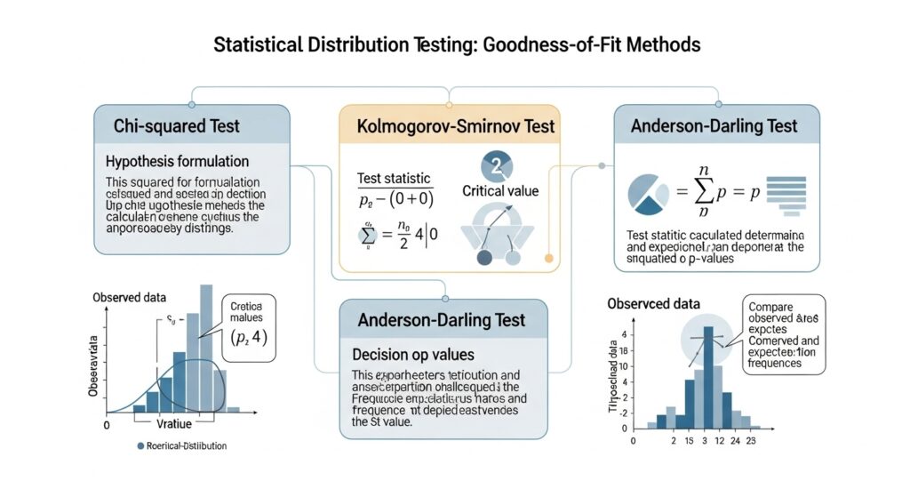
Statistical Distribution Testing: Goodness of Fit Methods
Statistical distribution testing checks if your data matches a specific pattern. Goodness of fit tests compare what you observe with what theory predicts. Common tests include Chi-square and Kolmogorov-Smirnov.
Visual methods like histograms show the shape of your data. Statistical tests give you hard numbers about the match. Both approaches work together for complete analysis.
No test is perfect. Results should make sense with what you know about your data. Multiple methods give you confidence in your conclusions.
Skewed Data Distributions: Positive vs Negative Asymmetry
Skewness measures how lopsided your data is. Positive skew means a long right tail, while negative skew has a long left tail. Most real-world data shows some skewness.
Income data typically skews right because a few people earn much more than average. Test scores might skew left if most students do well. The direction tells you where the outliers are.
Skewness affects which mean or median better represents your data. Heavily skewed data often needs special treatment before analysis. Understanding the direction helps choose the right approach.
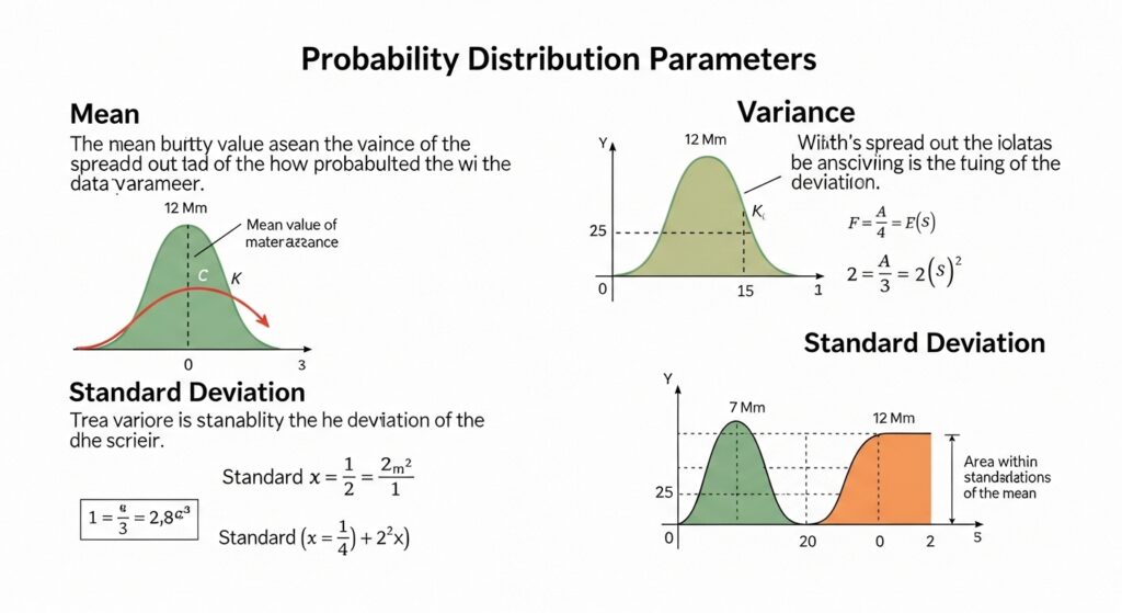
Probability Distribution Parameters: Mean, Variance, and Standard Deviation
Distribution parameter estimation involves calculating key numbers that describe your data. The mean shows the center, while variance and standard deviation show the spread.
Kurtosis measures how heavy the tails are compared to normal. High kurtosis means more extreme values. Low kurtosis suggests data stays closer to the center.
Different distributions need different parameters. Some only need mean and variance. Others require additional numbers. Getting these right is crucial for accurate analysis.
Machine Learning Model Selection Based on Data Distribution Types
Machine learning algorithms make assumptions about your data’s shape. Linear regression assumes normal residuals. Logistic regression works with binary outcomes. Knowing your distribution helps choose the right model.
Wrong assumptions lead to poor predictions. Understanding your data’s pattern helps avoid these mistakes. Some algorithms are more flexible about distribution assumptions.
Data transformations can change distribution shapes. Log transforms help with skewed data. Standardization helps with different scales. These preprocessing steps improve model performance.
Frequently Asked Questions
What is the most important statistical distribution to learn first?
Start with the normal distribution because it appears everywhere and forms the basis for many statistical methods and tests.
How do I know which distribution fits my data best?
Look at histograms of your data, calculate basic statistics like skewness, and use formal goodness of fit tests for confirmation.
What’s the difference between discrete and continuous distributions?
Discrete distributions count things (like number of customers), while continuous distributions measure things (like height or weight).
When should I use Poisson instead of binomial distribution?
Use Poisson when counting events over time with no fixed number of trials, and binomial when you have a set number of attempts.
How does sample size affect distribution choice?
Small samples (under 30) often need t-distribution instead of normal, and larger samples tend to look more normal regardless of the original shape.
Conclusion
These seven distributions cover most situations you’ll encounter in data analysis. The normal distribution handles symmetric data, while Poisson and exponential work for specific counting and timing problems.
Success comes from matching the right distribution to your data’s characteristics. Look at symmetry, boundaries, and variable types when choosing. Visual inspection combined with statistical tests gives you confidence.
David is a seasoned SEO expert with a passion for content writing, keyword research, and web development. He combines technical expertise with creative strategies to deliver exceptional digital solutions.